PyDiffGame is a Python implementation of a Nash Equilibrium solution to Differential Games, based on a reduction of Game Hamilton-Bellman-Jacobi (GHJB) equations to Game Algebraic and Differential Riccati equations, associated with Multi-Objective Dynamical Control Systems
The method relies on the formulation given in:
-
The thesis work "Differential Games for Compositional Handling of Competing Control Tasks" (Research Gate)
-
The conference article "Composition of Dynamic Control Objectives Based on Differential Games" (IEEE | Research Gate)
If you use this work, please cite our paper:
@conference{med_paper,
  author={Kricheli, Joshua Shay and Sadon, Aviran and Arogeti, Shai and Regev, Shimon and Weiss, Gera},
  booktitle={29th Mediterranean Conference on Control and Automation (MED)},
  title={{Composition of Dynamic Control Objectives Based on Differential Games}},
  year={2021},
  pages={298-304},
  doi={10.1109/MED51440.2021.9480269}}
To install this package run this from the command prompt:
pip install PyDiffGame
The package was tested for Python >= 3.10, along with the listed packages versions in requirments.txt
The package defines an abstract class PyDiffGame.py. An object of this class represents an instance of differential game.
The input parameters to instantiate a PyDiffGame object are:
-
A:np.arrayof shape$(n,n)$
System dynamics matrix
-
B:np.arrayof shape$(n, m_1 + ... + m_N)$ , optional
Input matrix for all virtual control objectives
-
Bs:Sequenceofnp.arrayobjects of len$(N)$ , each array$B_i$ of shape$(n,m_i)$ , optional
Input matrices for each virtual control objective
-
Qs:Sequenceofnp.arrayobjects of len$(N)$ , each array$Q_i$ of shape$(n,n)$ , optional
State weight matrices for each virtual control objective
-
Rs:Sequenceofnp.arrayobjects of len$(N)$ , each array$R_i$ of shape$(m_i,m_i)$ , optional
Input weight matrices for each virtual control objective
-
Ms:Sequenceofnp.arrayobjects of len$(N)$ , each array$M_i$ of shape$(m_i,m)$ , optional
Decomposition matrices for each virtual control objective
-
objectives:SequenceofObjectiveobjects of len$(N)$ , each$O_i$ specifying$Q_i, R_i$ and$M_i$ , optional
Desired objectives for the game
-
x_0:np.arrayof len$(n)$ , optional
Initial state vector
-
x_T:np.arrayof len$(n)$ , optional
Final state vector, in case of signal tracking
T_f: positivefloat, optional
System dynamics horizon. Should be given in the case of finite horizon
-
P_f:listofnp.arrayobjects of len$(N)$ , each array$P_{f_i}$ of shape$(n,n)$ , optional, default = uncoupled solution ofscipy's solve_are
Final condition for the Riccati equation array. Should be given in the case of finite horizon
-
state_variables_names:Sequenceofstrobjects of len$(N)$ , optional
The state variables' names to display when plotting
show_legend:boolean, optional
Indicates whether to display a legend in the plots
-
state_variables_names:Sequenceofstrobjects of len$(n)$ , optional
The state variables' names to display
-
epsilon_x:floatin the interval$(0,1)$ , optional
Numerical convergence threshold for the state vector of the system
-
epsilon_P:floatin the interval$(0,1)$ , optional
Numerical convergence threshold for the matrices P_i
L: positiveint, optional
Number of data points
eta: positiveint, optional
The number of last matrix norms to consider for convergence
debug:boolean, optional
Indicates whether to display debug information
To demonstrate the use of the package, we provide a few running examples. Consider the following system of masses and springs:
The performance of the system under the use of the suggested method is compared with that of a Linear Quadratic Regulator (LQR). For that purpose, class named PyDiffGameLQRComparison is defined. A comparison of a system should subclass this class.
As an example, for the masses and springs system, consider the following instantiation of an MassesWithSpringsComparison object:
import numpy as np
from PyDiffGame.examples.MassesWithSpringsComparison import MassesWithSpringsComparison

N = 2
k = 10
m = 50
r = 1
epsilon_x = 10e-8
epsilon_P = 10e-8
q = [[500, 2000], [500, 250]]

x_0 = np.array([10 * i for i in range(1, N + 1)] + [0] * N)
x_T = x_0 * 10 if N == 2 else np.array([(10 * i) ** 3 for i in range(1, N + 1)] + [0] * N)
T_f = 25

masses_with_springs = MassesWithSpringsComparison(N=N,
                                                  m=m,
                                                  k=k,
                                                  q=q,
                                                  r=r,
                                                  x_0=x_0,
                                                  x_T=x_T,
                                                  T_f=T_f,
                                                  epsilon_x=epsilon_x,
                                                  epsilon_P=epsilon_P)
Consider the constructor of the class MassesWithSpringsComparison:
import numpy as np
from typing import Sequence, Optional

from PyDiffGame.PyDiffGame import PyDiffGame
from PyDiffGame.PyDiffGameLQRComparison import PyDiffGameLQRComparison
from PyDiffGame.Objective import GameObjective, LQRObjective


class MassesWithSpringsComparison(PyDiffGameLQRComparison):
    def __init__(self,
                 N: int,
                 m: float,
                 k: float,
                 q: float | Sequence[float] | Sequence[Sequence[float]],
                 r: float,
                 Ms: Optional[Sequence[np.array]] = None,
                 x_0: Optional[np.array] = None,
                 x_T: Optional[np.array] = None,
                 T_f: Optional[float] = None,
                 epsilon_x: Optional[float] = PyDiffGame.epsilon_x_default,
                 epsilon_P: Optional[float] = PyDiffGame.epsilon_P_default,
                 L: Optional[int] = PyDiffGame.L_default,
                 eta: Optional[int] = PyDiffGame.eta_default):
        I_N = np.eye(N)
        Z_N = np.zeros((N, N))

        M_masses = m * I_N
        K = k * (2 * I_N - np.array([[int(abs(i - j) == 1) for j in range(N)] for i in range(N)]))
        M_masses_inv = np.linalg.inv(M_masses)

        M_inv_K = M_masses_inv @ K

        if Ms is None:
            eigenvectors = np.linalg.eig(M_inv_K)[1]
            Ms = [eigenvector.reshape(1, N) for eigenvector in eigenvectors]

        A = np.block([[Z_N, I_N],
                      [-M_inv_K, Z_N]])
        B = np.block([[Z_N],
                      [M_masses_inv]])

        Qs = [np.diag([0.0] * i + [q] + [0.0] * (N - 1) + [q] + [0.0] * (N - i - 1))
              if isinstance(q, (int, float)) else
              np.diag([0.0] * i + [q[i]] + [0.0] * (N - 1) + [q[i]] + [0.0] * (N - i - 1)) for i in range(N)]

        M = np.concatenate(Ms,
                           axis=0)

        assert np.all(np.abs(np.linalg.inv(M) - M.T) < 10e-12)

        Q_mat = np.kron(a=np.eye(2),
                        b=M)

        Qs = [Q_mat.T @ Q @ Q_mat for Q in Qs]

        Rs = [np.array([r])] * N
        R_lqr = 1 / 4 * r * I_N
        Q_lqr = q * np.eye(2 * N) if isinstance(q, (int, float)) else np.diag(2 * q)

        state_variables_names = ['x_{' + str(i) + '}' for i in range(1, N + 1)] + \
                                ['\\dot{x}_{' + str(i) + '}' for i in range(1, N + 1)]
        args = {'A': A,
                'B': B,
                'x_0': x_0,
                'x_T': x_T,
                'T_f': T_f,
                'state_variables_names': state_variables_names,
                'epsilon_x': epsilon_x,
                'epsilon_P': epsilon_P,
                'L': L,
                'eta': eta}

        lqr_objective = [LQRObjective(Q=Q_lqr,
                                      R_ii=R_lqr)]
        game_objectives = [GameObjective(Q=Q,
                                         R_ii=R,
                                         M_i=M_i) for Q, R, M_i in zip(Qs, Rs, Ms)]
        games_objectives = [lqr_objective,
                            game_objectives]

        super().__init__(args=args,
                         M=M,
                         games_objectives=games_objectives,
                         continuous=True)
Finally, consider calling the masses_with_springs object as follows:
output_variables_names = ['$\\frac{x_1 + x_2}{\\sqrt{2}}$',
                          '$\\frac{x_2 - x_1}{\\sqrt{2}}$',
                          '$\\frac{\\dot{x}_1 + \\dot{x}_2}{\\sqrt{2}}$',
                          '$\\frac{\\dot{x}_2 - \\dot{x}_1}{\\sqrt{2}}$']

masses_with_springs(plot_state_spaces=True,
                    plot_Mx=True,
                    output_variables_names=output_variables_names,
                    save_figure=True)
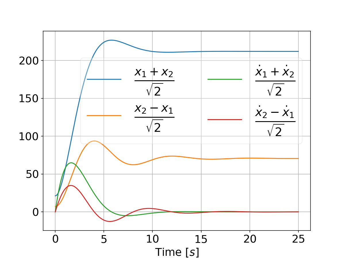
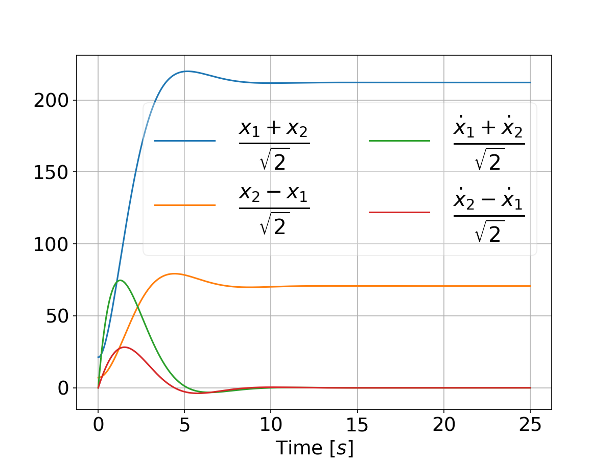
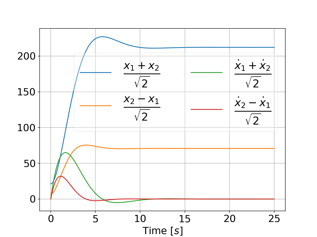
Refer This will result in the following plot that compares the two systems performance for a differential game vs an LQR:
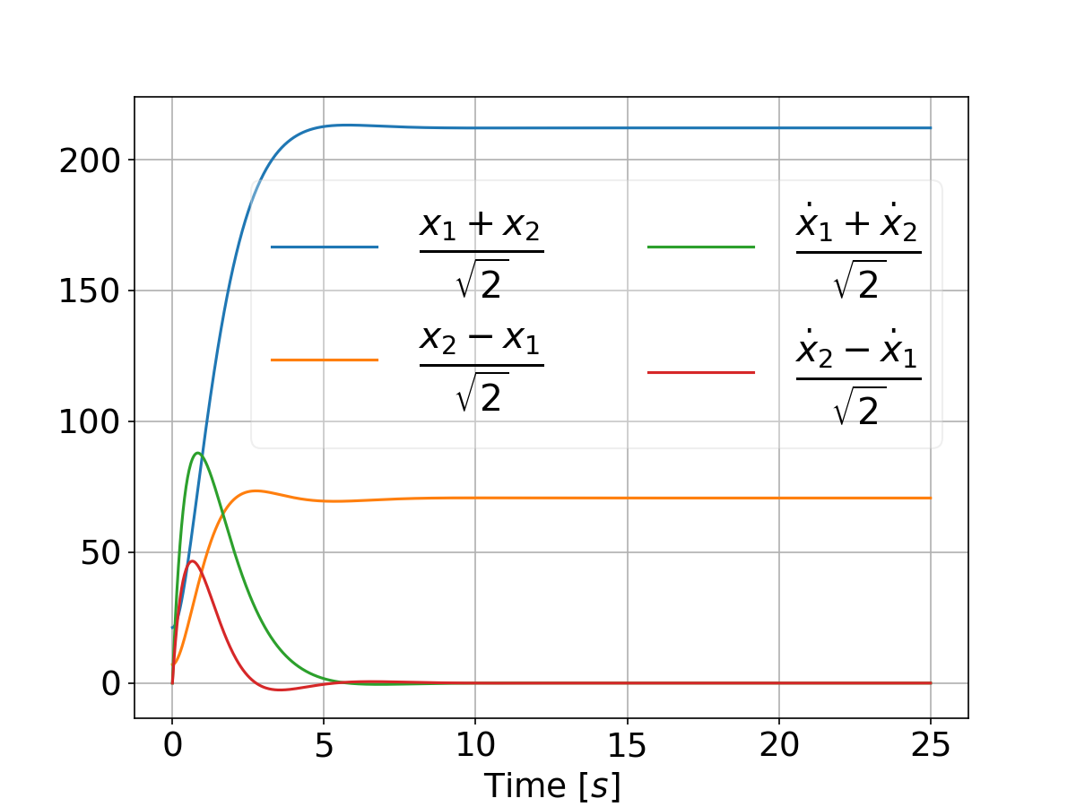
And when tweaking the weights by setting
qs = [[500, 5000]]we have:
This research was supported in part by the Leona M. and Harry B. Helmsley Charitable Trust through the Agricultural, Biological and Cognitive Robotics Initiative and by the Marcus Endowment Fund both at Ben-Gurion University of the Negev, Israel. This research was also supported by The Israeli Smart Transportation Research Center (ISTRC) by The Technion and Bar-Ilan Universities, Israel.


