The Bradford method is a popular biochemical technique for determining the concentration of protein.
A common kit like the Thermo Fisher Scientific (cat. no. 23236, http://bit.ly/2DaYy7C) uses the Coomassie Brilliant Blue G-250 dye molecule. In the presence the protein, a conformational state in the dye is stabilized resulting in a color change. The color change is proportional to the amount of protein and can be detected by a spectrophotometer reading absorbance at 595 nm.
PlyCB reacts with Dye
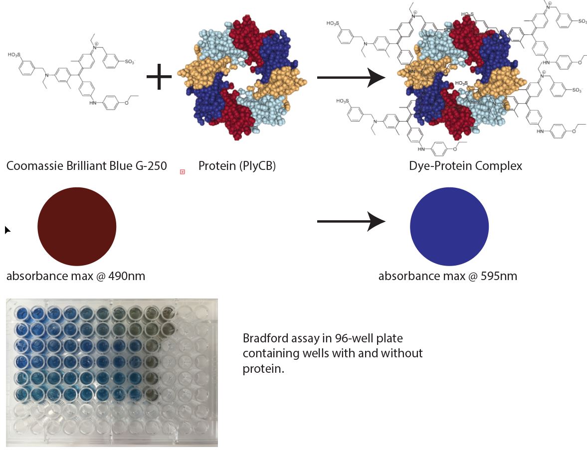
Precise protein concentration is an important characteristic for downstream experiments like ELISAs, protein-protein interactions and isothermal titration calorimetry.
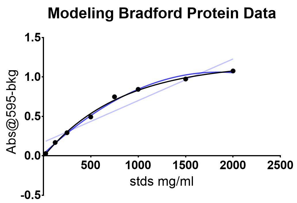
Although the dye and protein react in a proportional manner and can be characterized with a linear model, high concentrations of protein will stabilize most dye molecules causing saturation. Saturation causes a bowing in the data, and can be seen with the bovin serum albumin (BSA) standards recommended by the kit. The curve is better approximated by a non-linear regression method.
I was taught to use a linear model as it's simple and accurate for lower protein concentrations. However, a linear model results in greater error when calculating unknown high protein concentrations.
Other non-linear regression models like second-order polynomials can approximate the data but also can fail at the lower or higher ends. Growth curves or enzymatic models fit the data to an "S" curve.
I recently discovered that a one phase association model best approximates all standard-BSA protein concentrations recommended by the provider.
Y=(Y0 - Plateau)exp(-KX) + Plateau
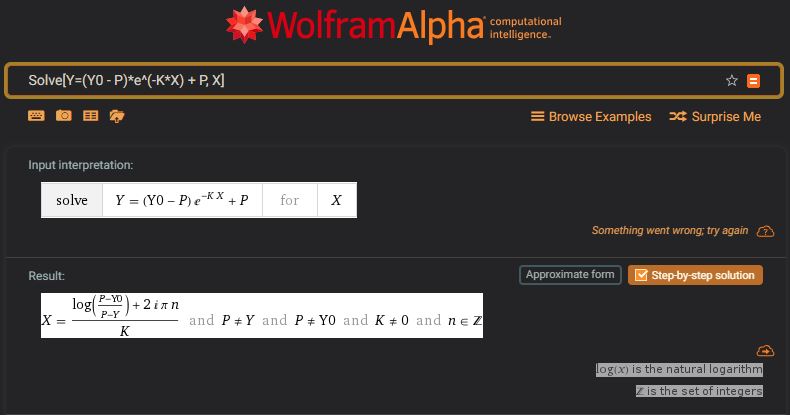
WA link: https://www.wolframalpha.com/input/?i=Solve%5BY%3D(Y0+-+P)*e%5E(-K*X)+%2B+P,+X%5D
The data was plotted and modeled with linear (lilac), polynomial (blue) and one-phase association models (black).
| mg/ml | abs |
|---|---|
| 2000 | 1.07685 |
| 1500 | 0.9741 |
| 1000 | 0.8432 |
| 750 | 0.74875 |
| 500 | 0.4937 |
| 250 | 0.2928 |
| 125 | 0.1696 |
| 25 | 0.02865 |
Data modeling down in GraphPad Prism. The one phase association was constrained to 0 as the background was subtracted from the absorbance values.
The purpose of creating a standard curve is so that unknown protein concentrations can be interpolated. Given absorbances (yi), what are the concentrations (xi)?
Solving the one-phase equation by hand for x I obtained: -[ln((y0+p-y)/p))]*1/k = x
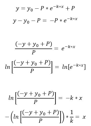
However, Wolfram Alpha has a different solution (above). Both solutions should be similar but there are differences for which I cannot yet account.
| mg/ml | abs | HK_eqn | WA_eqn |
|---|---|---|---|
| 2000 | 1.07685 | 2100 | 2006 |
| 1500 | 0.9741 | 1472 | 1431 |
| 1000 | 0.8432 | 1049 | 1028 |
| 750 | 0.74875 | 841 | 826 |
| 500 | 0.4937 | 454 | 448 |
| 250 | 0.2928 | 242 | 239 |
| 125 | 0.1696 | 135 | 134 |
| 25 | 0.02865 | 28 | 28 |
The data and Excel equations can be found in the Excel workbook in this repository.
- In the future I'd like to use scipy optimize curve fit to conduct least squares so that Excel and GraphPad will be unnecessary. Done [See Notebook in this repository.]
- I'd also like to explore this paper and linearization for the lower ends of the quantification
- Make a website so that values can be parsed and curve generated. Unknown samples can be easily interpolated.