Name
基于Nadaraya-Watson回归和ATR通道的趋势跟踪策略Trend-Following-Strategy-Based-on-Nadaraya-Watson-Regression-and-ATR-Channel
Author
ChaoZhang
Strategy Description
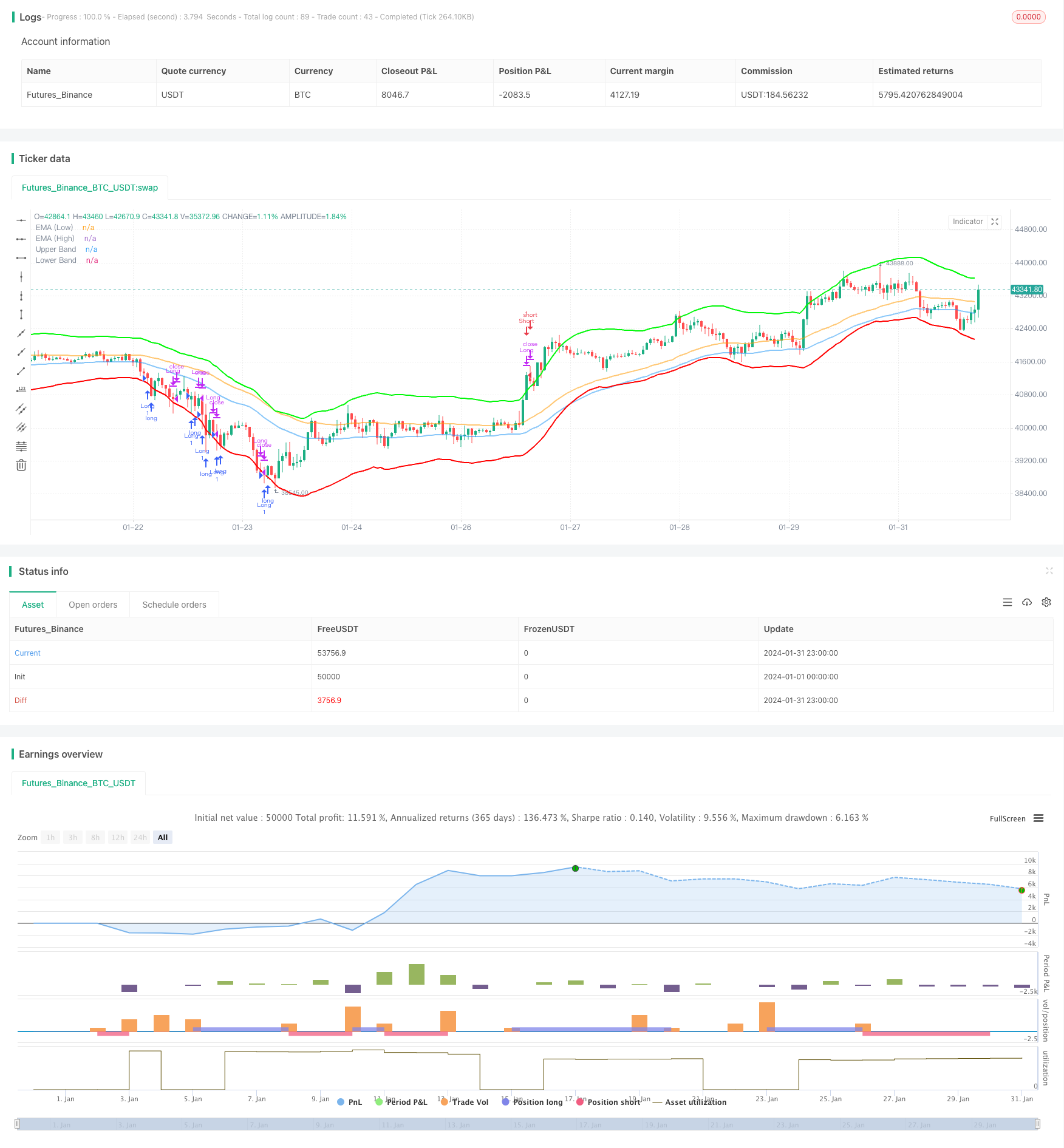
本策略是一种趋势跟踪策略,它结合了Nadaraya-Watson回归和ATR通道来识别趋势方向和入场点。当价格突破下轨时,做多;当价格突破上轨时,平仓。同时设置了止损机制。
首先,该策略使用 Nadaraya-Watson 核回归来计算两个不同滞后期的回归曲线,然后比较两条回归曲线的交叉来判断趋势方向。具体来说,分别计算 h期和 h-lag期的回归曲线,当 h-lag期曲线上穿 h期曲线时判断为看多;当 h-lag期曲线下穿 h期曲线时判断为看空。
其次,该策略使用ATR通道来确定入场点。上轨为回归曲线加上n期ATR的乘数,下轨为回归曲线减去n期ATR的乘数。当价格突破上轨时看空并入场,突破下轨时看多并入场。
最后,设置了止损机制。如果价格连续stopLossBars根K线低于入场价,则止损出场。
这种策略结合回归分析和通道 breakthrough,能比较准确地把握市场趋势的方向和力度。相比单一使用移动均线等指标识别趋势,这种方法减少了假信号,从而提高了策略的稳定性。
另外,ATR通道设置了合理的入场点,避免在趋势反转点附近错误入场。止损机制也有效控制了单笔损失。
所以,这种策略具有识别趋势能力强、出入场比较准确、单笔止损风险可控等优势。
这种策略最大的风险在于当突破ATR通道时,价格可能就是在做反转或者盘整,从而导致不适合入场或者入场后很快就止损出场。
另外,回归曲线和ATR通道都需要一定参数优化。如果参数设置不当,回归分析效果不佳,或者ATR幅度过大过小,都会影响策略的效果。
可以考虑结合其他指标判断趋势和反转信号,例如VOLUME,MACD等,以提高策略的稳定性和准确性。
回归分析中的核函数也可以调整,如考虑Epanechnikov核等,看是否能获得更好的拟合效果。
ATR通道的ATR周期和乘数也需要反复测试优化,找到最佳的参数组合。
本策略综合运用回归分析和通道突破方法,识别趋势方向和力度,在合理点位入场,并设置止损,从而实现稳定的趋势跟踪策略。次策略优化空间还很大,值得进一步测试改进。
||
This strategy is a trend following strategy that combines Nadaraya-Watson regression and ATR channel to identify trend direction and entry points. It goes long when price breaks through the lower rail and closes position when price breaks through the upper rail. A stop loss mechanism is also set.
Firstly, this strategy uses Nadaraya-Watson kernel regression to calculate two regression curves with different lags, and compares the crossover of the two curves to determine the trend direction. Specifically, it calculates the regression curves of h-period and h-lag-period respectively. When the h-lag-period curve crosses over the h-period curve, it indicates a long signal. When the h-lag-period curve crosses below the h-period curve, it indicates a short signal.
Secondly, this strategy uses ATR channel to determine entry points. The upper rail is the regression curve plus n-period ATR multiplier and the lower rail is the regression curve minus the n-period ATR multiplier. It goes long when price breaks through the lower rail and goes short when price breaks through the upper rail.
Finally, a stop loss mechanism is set. If the price stays below the entry price for stopLossBars consecutive bars, the position will be closed by stop loss.
This strategy combines regression analysis and channel breakthrough, which can capture the trend direction and momentum relatively accurately. Compared with using single indicators like moving average to identify trends, this method reduces false signals and thus improves the stability of the strategy.
In addition, the ATR channel sets reasonable entry points, avoiding wrong entries around trend reversal points. The stop loss mechanism also effectively controls the single loss.
Therefore, this strategy has advantages like strong ability to identify trends, relatively accurate entries and exits, controllable single stop loss risk, etc.
The biggest risk of this strategy is that when price breaks through the ATR channel, it may just be making a reversal or consolidation, which leads to improper entry or quick stop loss after entry.
In addition, both the regression curves and ATR channels need some parameter optimization. Improper parameter settings may lead to poor regression analysis results or over-wide or over-narrow ATR ranges, which will affect the performance of the strategy.
We can consider combining other indicators to judge trend and reversal signals, such as VOLUME, MACD etc. to improve the stability and accuracy of the strategy.
The kernel function in the regression analysis can also be adjusted, such as trying Epanechnikov kernel, to see if better fitting effects can be obtained.
The ATR period and multiplier of the ATR channel also need repeated testing and optimization to find the best parameter combination.
This strategy combines the use of regression analysis and channel breakthrough to identify trend direction and strength, enters at reasonable points, and sets stop loss, thus realizing a stable trend following strategy. There is still a large room for further testing and improvement of this strategy.
[/trans]
Strategy Arguments
| Argument | Default | Description |
|---|---|---|
| v_input_1_close | 0 | Source: close |
| v_input_2 | 10 | Lookback Window |
| v_input_3 | 10 | Relative Weighting |
| v_input_4 | 50 | Start Regression at Bar |
| v_input_5 | 2 | Lag |
| v_input_6 | 3 | Stop Loss Bars |
| v_input_7 | 46 | EMA Period |
| v_input_8 | 32 | ATR Period |
| v_input_9 | 2.7 | Multiplier |
Source (PineScript)
/*backtest
start: 2024-01-01 00:00:00
end: 2024-01-31 23:59:59
period: 1h
basePeriod: 15m
exchanges: [{"eid":"Futures_Binance","currency":"BTC_USDT"}]
*/

//@version=5
strategy("Custom Strategy with Stop Loss and EMA", overlay=true)

src = input(close, title='Source')
h = input(10, title='Lookback Window', tooltip='The number of bars used for the estimation.')
r = input(10, title='Relative Weighting', tooltip='Relative weighting of time frames.')
x_0 = input(50, title='Start Regression at Bar',  tooltip='Bar index on which to start regression.')
lag = input(2, title='Lag', tooltip='Lag for crossover detection.')
stopLossBars = input(3, title='Stop Loss Bars', tooltip='Number of bars to check for stop loss condition.')
emaPeriod = input(46, title='EMA Period',  tooltip='Period for Exponential Moving Averages.')

lenjeje = input(32, title='ATR Period', tooltip='Period to calculate upper and lower band')
coef = input(2.7, title='Multiplier', tooltip='Multiplier to calculate upper and lower band')

// Function for Nadaraya-Watson Kernel Regression
kernel_regression1(_src, _size, _h) =>
    _currentWeight = 0.0
    _cumulativeWeight = 0.0
    for i = 0 to _size + x_0
        y = _src[i]
        w = math.pow(1 + (math.pow(i, 2) / ((math.pow(_h, 2) * 2 * r))), -r)
        _currentWeight += y * w
        _cumulativeWeight += w
    [_currentWeight, _cumulativeWeight]

// Calculate Nadaraya-Watson Regression
[currentWeight1, cumulativeWeight1] = kernel_regression1(src, h, h)
yhat1 = currentWeight1 / cumulativeWeight1
[currentWeight2, cumulativeWeight2] = kernel_regression1(src, h-lag, h-lag)
yhat2 = currentWeight2 / cumulativeWeight2

// Calculate Upper and Lower Bands
upperjeje = yhat1 + coef * ta.atr(lenjeje)
lowerjeje = yhat1 - coef * ta.atr(lenjeje)

// Plot Upper and Lower Bands
plot(upperjeje, color=color.rgb(0, 247, 8), title="Upper Band", linewidth=2)
plot(lowerjeje, color=color.rgb(255, 0, 0), title="Lower Band", linewidth=2)

// Calculate EMAs
emaLow = ta.ema(low, emaPeriod)
emaHigh = ta.ema(high, emaPeriod)

// Plot EMAs
plot(emaLow, color=color.rgb(33, 149, 243, 47), title="EMA (Low)", linewidth=2)
plot(emaHigh, color=color.rgb(255, 153, 0, 45), title="EMA (High)", linewidth=2)

// Long Entry Condition
longCondition = low < lowerjeje
strategy.entry("Long", strategy.long, when=longCondition)

// Stop Loss Condition
stopLossCondition = close[1] < strategy.position_avg_price and close[2] < strategy.position_avg_price and close[3] < strategy.position_avg_price
strategy.close("Long", when=stopLossCondition)

// Close and Reverse (Short) Condition
shortCondition = high > upperjeje
strategy.close("Long", when=shortCondition)
strategy.entry("Short", strategy.short, when=shortCondition)
Detail
https://www.fmz.com/strategy/442511
Last Modified
2024-02-22 15:15:03
