-
Notifications
You must be signed in to change notification settings - Fork 0
/
Copy pathREADME.Rmd
156 lines (104 loc) · 4.97 KB
/
README.Rmd
1
2
3
4
5
6
7
8
9
10
11
12
13
14
15
16
17
18
19
20
21
22
23
24
25
26
27
28
29
30
31
32
33
34
35
36
37
38
39
40
41
42
43
44
45
46
47
48
49
50
51
52
53
54
55
56
57
58
59
60
61
62
63
64
65
66
67
68
69
70
71
72
73
74
75
76
77
78
79
80
81
82
83
84
85
86
87
88
89
90
91
92
93
94
95
96
97
98
99
100
101
102
103
104
105
106
107
108
109
110
111
112
113
114
115
116
117
118
119
120
121
122
123
124
125
126
127
128
129
130
131
132
133
134
135
136
137
138
139
140
141
142
143
144
145
146
147
148
149
150
151
152
153
154
155
---
output: github_document
bibliography: references.bib
---
<!-- README.md is generated from README.Rmd. Please edit that file -->
```{r, include = FALSE}
knitr::opts_chunk$set(
collapse = TRUE,
comment = "#>",
fig.path = "man/figures/README-",
out.width = "100%"
)
```
# biomech
<!-- badges: start -->
[](https://github.com/PalmStudio/biomech/actions)
<!-- badges: end -->
`biomech` aims at computing bending and torsion of beams following the Euler-Bernoulli beam theory. It is specifically designed to be applied on
tree branches (or e.g. palm leaves), but can be applied to any other beam-shaped structure.
## Table of Contents
* [1. Installation](#1-installation)
* [2. Examples](#2-examples)
* [2.1 Example field data](#21-example-field-data)
* [2.1.1 Presentation](#211-presentation)
* [2.1.2 Un-bending](#211-un-bending)
* [2.2 Bending model](#22-bending-model)
* [2.3 Plotting](#23-plotting)
* [2.4 Optimization](#24-optimization)
* [3. References](#3-references)
## 1. Installation
You can install biomech from [GitHub](https://github.com/) with:
``` r
# install.packages("devtools")
devtools::install_github("PalmStudio/biomech")
```
## 2. Examples
The bending function (`bend()`) uses two parameters: the elastic modulus, and the shear modulus. A good introduction to these concepts is available on [wikipedia](https://en.wikipedia.org/wiki/Euler%E2%80%93Bernoulli_beam_theory)
In our examples, these parameters are unknown at first, but they can be computed from field data.
### 2.1 Example field data
#### 2.1.1 Presentation
Our field data consist on measurements made along the leaf of a palm plant. The leaf is discretized into 5 segments. each segment is defined by a single point at the beginning of the segment representing its cross-section, with attributes such as its dimensions (width, height) and shape (=`type`), the distance from the last point to the current point, the inclination and torsion at the first point, the x, y and z positions of the point (used to cross-validate), the mass of the rachis and of the leaflets on the right and on the left separately.
Here is a little depiction of the information:
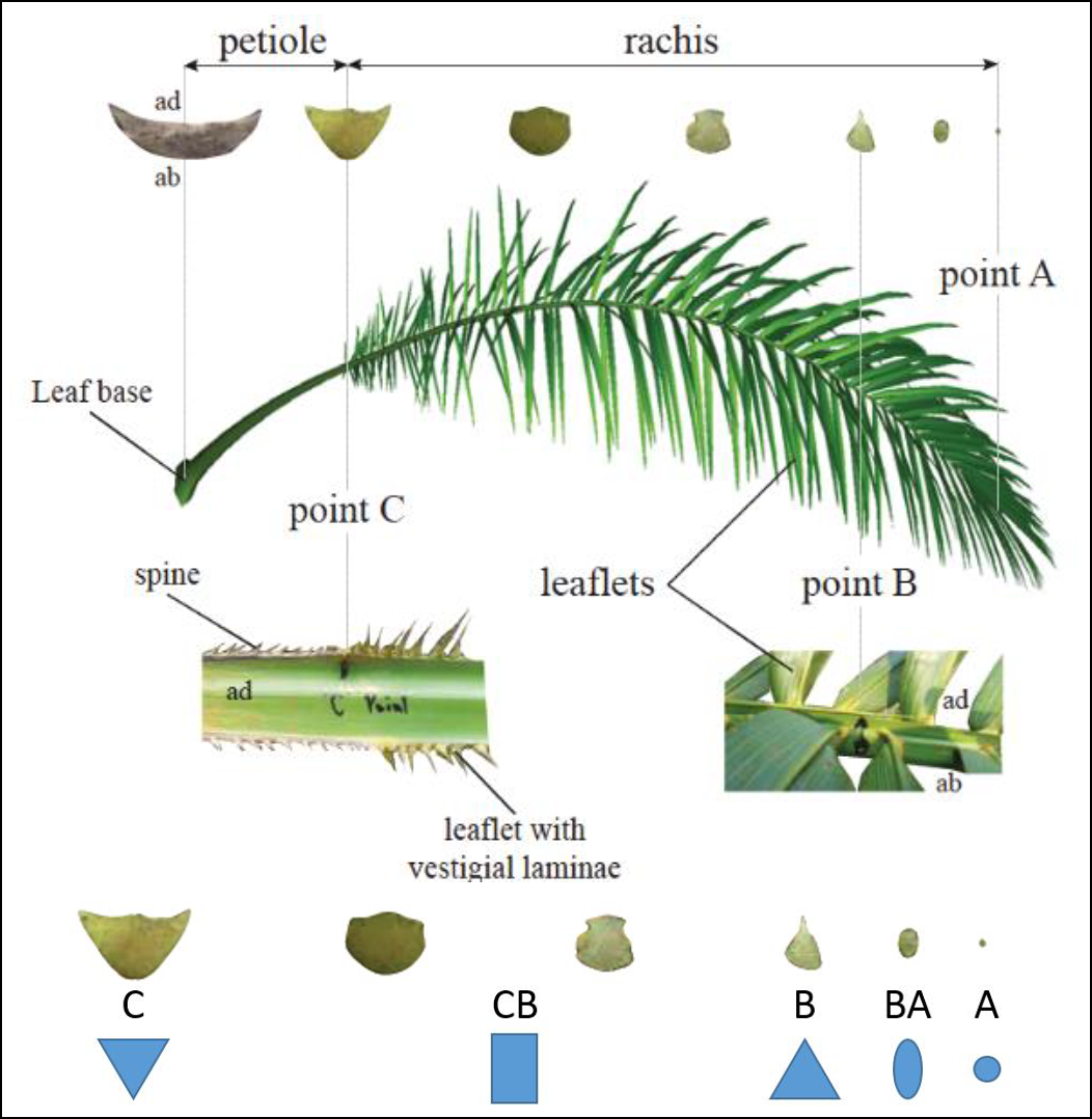
See [@perezAnalyzingModellingGenetic2017] for more information about the subject.
The example field data is available from the package and can be read using:
```{r example}
library(biomech)
file_path = system.file("extdata/6_EW01.22_17_kanan.txt", package = "biomech")
field_data = read_mat(file_path)
```
Here is what it looks like:
```{r echo=FALSE}
field_data
```
#### 2.1.2 Un-bending
We can use the field data to try our bending model. But first, it must be "un-bent" back to a straight line. This is made using `unbend()`, such as:
```{r}
# Un-bending the field measurements:
df_unbent = unbend(field_data)
```
### 2.2 Bending model
We can use `bend()` to bend a straight beam providing initial values and known elastic and shear modulus.
We can try it out on our example leaf data. But first, we have to compute a variable that is missing from our `df_unbent` data.frame: the distance of application of the mass of the leaflets on the right and left sides of each segment. We can approximate this using a sine function:
```{r}
# Adding the distance of application of the left and right weight (leaflets):
df_unbent$distance_application = distance_weight_sine(df_unbent$x)
```
Know we're ready to go with our model, using some expert knowledge to estimate the elastic and shear modulus:
```{r}
# (Re-)computing the deformation:
df_bent = bend(df_unbent, elastic_modulus = 2000, shear_modulus = 400)
```
### 2.3 Plotting
We can now plot the results using `plot_bending()`. We want to compare the observed data with the simulated data. We also want to check if the straight line was right. Let's put all three on a single plot:
```{r}
plot_bending(Observed = field_data, "Un-Bent obs." = df_unbent, Modeled = df_bent)
```
We can even make a 3d plots using `plot_bent_3d()`:
```{r eval=FALSE}
plot_bending_3d(Observed = field_data, "Un-Bent obs." = df_unbent, Modeled = df_bent)
```
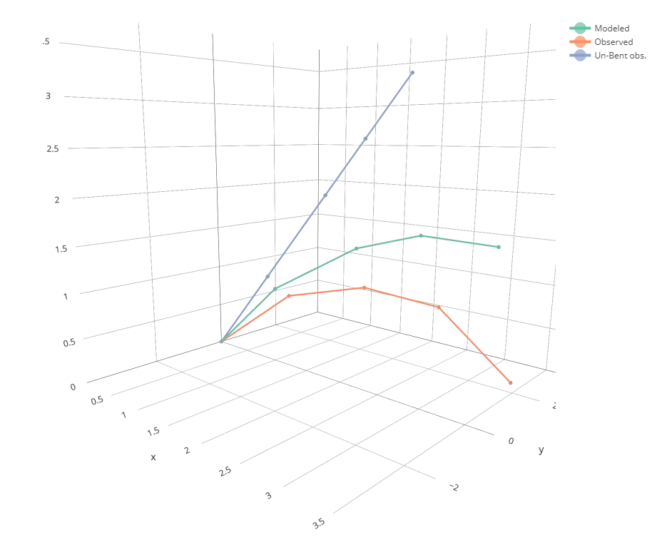
OK, not bad. But the adjustment is not really that close to the measurement.
### 2.4 Optimization
`optimize_bend()` can help us find out the right values for both our parameters:
```{r eval=TRUE}
params = optimize_bend(field_data, type = "all")
```
```{r include=FALSE}
# params = list(elastic_modulus = 1209.396, shear_modulus = 67.44096)
```
Here are our optimized values:
```{r}
params
```
And here is a the resulting plot:
```{r}
df_bent_optim = bend(df_unbent, elastic_modulus = params$elastic_modulus,
shear_modulus = params$shear_modulus)
plot_bending(Observed = field_data, "Un-Bent obs." = df_unbent,
Modeled = df_bent,
"Modeled (optimized)" = df_bent_optim)
```
## 3. References